
Saturation of Warming by the Greenhouse Gas CO2
W. Happer
Professor of Physics Emeritus, Princeton University, USA
L. Klett
Education and Outreach Manager, The CO2 Coalition
October 27, 2026
At current atmospheric concentrations C of carbon dioxide (CO2), there is less and less increase of the temperature T as more and more of the greenhouse gas CO2 is added. This law of diminishing returns is called saturation in radiation-transfer physics.
We will quote concentrations C in units of CO2 molecules per million air molecules, or ppm. It is useful to define a dimensionless relative concentration of CO2 by

where the saturation concentration,

which was discussed in reference [1]. For concentrations C ≪ δC, the CO2-induced greenhouse warming is very small but it is proportional to C. For C ≫ δC, the warming is proportional to log2(C/δC), where log2 is the base-2 logarithm function, for example log2(1) = 0, log2(2) = 1, log2(4) = 2, etc. It is also useful to define a dimensionless relative warming

Here we will take temperature sensitivity to be [1]

As discussed in reference [1], saturation can be summarized by a simple formula that gives the relative warming t in terms of the relative concentration c of CO2,

The inverse of (5) is

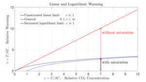
Figure 1: The relative warming t of (3) versus the relative concentration c of (1), as given by: (1) the high-concentration, saturated approximation (7); the generally correct formula (5); (3) the low-concentration, unsaturated approximation (9). As shown in (8), in the current year, 2026, atmospheric concentrations of CO2, C = 430 ppm, corrrespond to a relative concentration (1) of c = 1100. So current warmings are very well described by the high-concentration, logarithmic limit (7).
For the limit of very large relative concentrations, c ≫ 1, we can approximate the general warming formula (5) by

In the year 2026, the CO2 concentration C and its relative value c of (1) are approximately

Then the exact value of (5) is t = log2(1 + c) = log2(1101) = 10.1046 and the approximate value (7) is t = log2(c) = log2(1100) = 10.1033. Therefore, at the present time, the year 2026, (7) is a very good approximation to (5). The logarithmic formula (7) fails completely for c ≤ 1 since it gives negative relative warming, t < 0, and it implies an infinite negative warming as the CO2 concentration drops to zero. As c → 0 in (7), t = log2(c) → −∞.
To find a limiting expression for (5) for c ≪ 1, analogous to the approximation (7) for c ≫ 1, we write (5) as

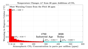
Figure 2: The warmings, ∆Tn from successive additions of ∆C = 20 ppm increments of CO2 to the atmosphere. The concentration after the first addition is C1 = 20 ppm, after the second addition, C2 = 40 ppm, etc. Over half of the total warming by the year 2026, Tn = 5.44 C, when the concentration was Cn = 420 ppm, was due to the first 20 ppm addition of CO2, which caused a warming of ∆T1 = 3.08 ◦C. Representative numerical values are shown in Table 1.
Here ln(x) = loge(x) is the natural, base-e logarithm of the variable x. In writing the second line of (9) we used the power series expansion

and we noted the identity

For example, if c = 0.01 the exact warming from (5) is t = log2(1.001) = 1.44 × 10⁻³ and the approximation (9) gives same number.
The general formula (5) for the relative warming t caused by the relative CO2 con-centration c is plotted in Fig. 1, along with the large-concentration limit (7) and small-concentration limit (9). In the year 2026, when the relative concentration is approximately c = 1100, according to (8), using the small-concentration warming formula (9), which does not account for saturation, instead of the correct general formula (5) that does, would exaggerate the predicted warming by a factor

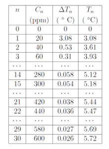
Table 1: The number n of concentration increments, ∆C = 20 ppm, added to the atmosphere is shown in the first column. The second column shows the cumulative concentration Cn of (14). The third column shows the incremental warming ∆Tn of (19), caused by adding the nth increment, ∆C = 20 ppm, of CO2. The fourth column shows the cumulative warming Tn of (18). Fig. 2 is a graphical display of the numbers in this table.
To write the second line of (12) we used (11).
Imagine that we increase the concentration of CO2 in equal 20 ppm increments,

After n increments, starting from C0 = 0, the concentration would be

The relative concentrations would be

where the saturation ratio is

Substituting (15) into (5) we see that adding n increments ∆C of (13) would increase the relative temperature by

From (17) and (3) we see that the temperature increase in degrees would be

Using (18) we see that the temperature increment caused by adding the nth increment (13) to the atmosphere would be
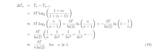
The second line of (19) is exact for n = 1, 2, 3, 4, . . .. The third line of (19) is a very good approximation to the second for n = 2, 3, 4, . . ., because r ≫ 1 in accordance with (16). In the fourth line we used the power series expansion (10).
Fig. 2 shows the incremental warmings ∆Tn of (19) caused by the nth addition of ∆C = 20 ppm to the atmosphere. Also shown are the cumulative CO2 concentrations Cn of (14) after the nth addition, and the cumulative warming temperatures Tn of (18). More than half of the warming in the year 2026, when the CO2 concentration is approximately C = 430 ppm, has been caused by the first 20 ppm increase in the concentration of CO2 from a vanishing initial concentration C0 = 0. Current additions of CO2 have very little effect because of the heavy saturation. Table 1 gives numerical values of some of the data plotted in Fig. 2.
References
[1] Saturation Graphics,
https: //co2coalition.org/publications/saturation-graphics/
Download Saturation of Warming by the Greenhouse Gas CO2 here: