W. A. van Wijngaarden
Department of Physics and Astronomy, York University, Canada

W. Happer
Department of Physics, Princeton University, USA

October 8, 2025

A graphic that has turned out to be helpful for explaining why doubling greenhouse gases has only a tiny effect on thermal radiation to space is a variant of Fig. 4 of our arXiv paper[1], which we show here as Fig. 1. The quantity plotted is the spectral flux, ˜ Z(ν,C), at the top of the cloud-free atmosphere. As indicated, the spectral flux depends on the CO2 concentration C (in ppm) and on the spatial frequency ν (in waves per cm) of the radiation. The total radiation to space, the areas under the curves are the frequency-integrated fluxes,

As indicated in Fig. 1, the frequency-integrated fluxes for the three concentrations of CO2 are

Increasing the concentration C of CO2 decreases the radiation to space. Averaged over Earth’s surface and time, the thermal radiation to space carries away the same amount of energy as is absorbed from sunlight. If the solar heating remains the same after an increase of CO2 concentration and decrease of flux to space, the Earth’s surface will have to warm to restore the flux and keep the solar heating rate equal to the thermal infrared cooling rate. From (2) – (4) we see that the first 400 ppm of CO2 added to an initially CO2-free atmosphere decreases the flux to space by 30 W m−2. A second addition of 400 ppm, raising the total concentration to 800 ppm, only decreases the flux by an additional 3 W m−2. As shown in the arXiv paper[1], every doubling of CO2 concentrations decreases the flux by

The equal decrease in flux to space for every doubling of the CO2 concentration, or “logarithmic” response works for concentrations between about C = 1 ppm and C = 10, 000 ppm, or for about 13 doublings from 1 ppm.

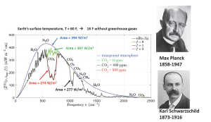
Figure 1: Radiation flux to space, ˜ Z(ν,C), from the top of the atmosphere as a function of spatial frequency ν (waves per cm) of the thermal radiation. The calculated values are for a summertime, temperate latitude and a surface temperature of 288.7 K. We have noted the spatial frequencies where the atmospheric opacity is dominated by the five major greenhouse gases, water vapor H2O, carbon dioxide, CO2, ozone O3, methane, CH4, and nitrous oxide, N2O. The black curve is the solution to the Schwarzschild equation for radiative transfer for C = 400 parts per million (ppm) of CO2, close to the present concentration. The red curve is for double that amount, C = 800 ppm, but for the same profiles of atmospheric temperature and other greenhouse gases concentrations. The green curve is for no CO2 at all. The smooth blue curve is the Planck flux for the same temperature, that is, the radiation that would reach space if there were no greenhouse gases at all and the surface had maximum thermal emissivity, ϵ = 1.

We can define the total radiative forcing, F(C), due to a concentration C of CO2 as

From (2)–(5) we see that three explicit values of the forcing are

A simple empirical formula for the forcing, F = F(C), that fits detailed calculation of the forcing well for 1 ppm < C < 10,000 ppm is

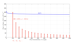
Figure 2: The blue curve is the radiative flux to space, Z(C), given by (12), versus the concentration C of carbon dioxide. The flux decreases rapidly with C for the first 100 ppm of CO2, but the rate of decrease slows down for higher concentrations. The vertical red lines show the flux decreases caused by 50 ppm increases of C for the sequence of values, [C0,C1,C2,C3, . . .] = [0, 50, 100, 150, . . .] ppm. Each additional 50 ppm increase has less effect than the previous one. For example, we see from the figure that the height of the first red bar, characterized by i = 2, is approximately 300 W m−2. So increasing the CO2 concentration from C1 = 50 ppm to C2 = 100 ppm decreases the flux to space by 300 W m−2/100 = 3 W m−2, in agreement with (5), since CO2 concentrations have doubled.

Using (8) to set F = 30 W m−2, C = 400 ppm and (5) to ΔF = 3 W m−2, we solve (10) for C0 to find

We use (6) and (10) to approximate the flux to outer space as

In Fig. 2 we have plotted (12) as the blue line, and we have plotted increments Z(C−ΔC)− Z(C) = F(C) − Z(C − ΔC) for equal increments ΔC = 50 ppm of CO2 concentration as the vertical red lines. The literature is replete with plots similar to the red vertical lines, but the blue line, the flux to space with no suppressed zero, is little known, and may clarify how small the forcing change is when the CO2 concentration increases from 400 ppm to 800 ppm.

Note that we are plotting fluxes and flux changes in Fig. 2, not temperature changes. This has the advantage that our results are almost the same as the most carefully calculated results of the climate-alarm establishment[1]. So it would be awkward for the establishment to deny that “instantaneous”, very large changes of CO2 concentration cause very small changes of flux to space. But people are interested in temperature changes, not flux changes. This is where all the mischief from positive feedback arises. Without huge positive feedbacks, ΔF = 3 W m−2 of clear-sky forcing only gives about 1 C of surface warming. Changes in water vapor and clouds are likely to significantly diminish the temperature changes due to changes in greenhouse gases, since most feedbacks in nature are negative. As shown in Fig. 2, adding CO2 to the atmosphere causes a very rapid decrease of flux to space, Z(C), for an atmosphere that starts with no CO2, C = 0. The decrease with increasing C then slows down dramatically so the blue curve of Fig. 2 is almost horizontal up to 1000 ppm. This is a familiar phenomenon to astronomers who work with radiation transfer from stars. It is called “saturation.” A good definition of saturation for the field of radiation transfer was given by Gussman [2]

“Saturation in a Fraunhofer line means that with increasing absorption the depression in the line (line depth) is no longer proportional to the optical thickness of the absorbing layer, as in the case of weak absorption.”

A perceptive astronomer looking at Fig. 1 would say that Earth’s thermal emission spectrum has a prominent Fraunhofer line from CO2, analogous to the yellow “D Fraunhofer line” of the Sun.

The word “saturation” means different things in different scientific fields. For example, if you add 360 grams of table salt crystals to a kilogram of water at room temperature (about 1 liter), the salt will dissolve completely to give a “saturated” solution. If you add 1000 grams of salt to a kilogram of water, only 360 grams will dissolve and 640 grams will remain as solid crystals on the bottom of the container. Adding more salt to a saturated solution has no effect on the amount of salt in solution. Adding more CO2 to the atmosphere, when its effects on radiation transfer are saturated, continues to decrease flux to space. But the decrease gets smaller and smaller as more CO2 is added.

References

[1] W. A. van Wijngaarden and W. Happer, Dependence of Earth’s Thermal Radiation on Five Most Abundant Greenhouse Gases https://arxiv.org/pdf/2006.03098.pdf

[2] A. E. Gussman, Saturation in Fraunhofer Lines, The Observatory, 87, 233-236 (1967), https://articles.adsabs.harvard.edu//full/1967Obs….87..233G/0000233. 000.html

Download the pdf here: Saturation