William Happer, Ph.D., Physics

Gregory Wrightstone, M.S., Geology

Frits Byron Soepyan, Ph.D., Chemical Engineering

August 21, 2026

Assuming that any human-caused increase of atmospheric CO2 concentration decays exponentially to zero, with a time constant of about 50 years, gives modelled concentrations that agree very well with observed concentrations and emissions. Figure 1 shows observed [1] human emissions of CO2, mostly due to combustion of fossil fuels, for the years 1850 to 2024. We will denote the years by the symbol tj , where

The data of Fig. 1 is from the spreadsheet of reference [1], column HX, lines 13-187.

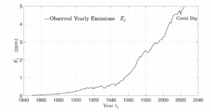
Figure 1: Yearly human emissions Ej from (5) of CO2 to the atmosphere in parts per million (ppm) versus calendar year tj of (1). The observational data is from reference [1]. Note the small dip in emissions in the year 2020 due to the Covid pandemic.

Examples of these data, in grams of carbon per year, are

The total number of molecules in Earth’s atmosphere is [2]

The mass of a carbon atom is

Therefore a mass increment Mj of carbon, added to the atmosphere as CO2 molecules in the year tj , would increase the concentration of CO2 by

We find good agreement with observed atmospheric CO2 concentrations if we assume that

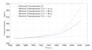
Figure 2: Atmospheric concentrations of CO2 in parts per million (ppm) versus calendar year, tj . The observed concentrations, C¯j , shown as the continuous blue line, are from references [3, 4]. The modeled concentrations Cj (τ) are from (7) and the annual emissions Ej of Fig. 1. For a decay time of τ = 50 y, the modeled concentrations, Cj(50 y) , shown as the dotted red line, are nearly the same as the observed concentrations. Neither observed nor modeled concentrations are influenced much by the “covid dip,” shown in Fig. 1.

the increment Ej of the CO2 added in the year j decays exponentially with a time constant τ of about 50 years,

Then in the year j, the concentration Cj in the atmosphere would be

where we take the pre-industrial concentration to be

The concentrations of CO2 modelled with (7) are shown in Fig. 2 for several possible decay times τ . Also shown are the observed concentrations ¯ Cj over the same time period, 1850 to 2024. The data from 1850 to 1958 [3] are from ice cores, and the data for 1959 to 2024 [4] are atmospheric observations. Representative values of the observed concentrations ¯ Cj are

As one can see from Fig. 2, assumed decay times τ shorter than 50 years give atmospheric CO2 concentrations smaller than those observed. Assumed decay times longer than 50 years give concentrations higher than those observed.

This extremely simple, 1-parameter (τ ) model gives very good agreement with observations for τ = 50 years. This is strong additional evidence that most of the increase of atmospheric CO2 over the past two centuries has been due to human emissions, as discussed in more depth in reference [5].

References

[1] Global Carbon Emissions, https://globalcarbonbudget.org/download/2371/?tmstv=176281725

[2] D. Alexander et al. Livestock, Methane and Climate https://co2coalition.org/publications/livestock-methane-and-climate/

[3] Ice core concentrations, 1850-1958, https://data.giss.nasa.gov/modelforce/ghgases/Fig1A.ext.txt

[4] Mauna Loa observations, 1959-2024, https://gml.noaa.gov/webdata/ccgg/trends/co2/co2_annmean_mlo.txt

[5] F. Engelbeen, R. Hannon and D. Burton, The Human Contribution to Atmospheric Carbon Dioxide, https://co2coalition.org/wp-content/uploads/2024/12/ Human-Contribution-to-Atmospheric-CO2-digital-compressed.pdf

Download the full publication here: Emission-Concentration 2026-08-21