Featured Photo: CO2 Coalition Member Andy May delivering keynote speech, August 30, 2022

By Andy May

This is the transcript, with minor edits to get it into blog post format, of my keynote speech to the Division of Professional Affairs, at the second International Meeting for Applied Geoscience and Energy Convention in the George R. Brown Convention Center in Houston on August 30, 2022.

In the great climate change debate between Princeton Professor, emeritus, William Happer and University of Melbourne Professor David Karoly, they were asked the following question by the moderator, James Barham:

“The IPCC’s official position may be summarized as making four claims: global warming is a well-established fact; it is anthropogenic; it is a major problem for humanity; and concerted global governmental action is required to combat it.”

James Barham and TheBestSchools.org

In this talk we will only cover a portion of the second and third parts of the question, which we rephrase as “Is burning fossil fuels and emitting CO₂ and other greenhouse gases to the atmosphere a good thing, or a bad thing for humanity.” The other facets of the question are well covered in my latest book. Much of this talk is from Chapter 10.

In answer to the question, Professor Happer wrote:

“There is no scientific evidence that global greenhouse gas emissions will have a harmful effect on climate. Quite the contrary, there is very good evidence that the modest increase in atmospheric CO₂ since the start of the Industrial age has already been good for the Earth and that more will be better.”

Professor William Happer

David Karoly’s response:

“Science has established that it is virtually certain that increases of atmospheric CO₂ due to burning of fossil fuels will cause climate change that will have substantial adverse impacts on humanity and on natural systems. Therefore, immediate, stringent measures to suppress the burning of fossil fuels are both justified and necessary.”

Professor David Karoly

By “Science,” Karoly means the views and opinions of the IPCC and other organizations that believe anthropogenic climate change is dangerous. Science is organized debate, both sides present their data and analysis, and eventually one side is found to be correct by comparing their projections to future observations, rinse, and repeat. Science is not a thing, a person, peer review, or consensus; it is a process. Scientific theories are validated by observations, not the opinions of scientists or government officials.

The two views presented above, both by very qualified and respected climate scientists, are mutually exclusive, which is correct? We will examine the data as it exists today, and you can decide. Observations support Happer’s view. Model projections of future climate support Karoly’s view in extreme scenarios. What is the cost of eliminating or curtailing fossil fuels? Is it cheaper and more reasonable to adapt to climate change? All good questions.

Karoly relies a lot on the IPCC. Just how much warming is dangerous? They claim that 1.5°C over the pre-industrial (pre-1750) temperature could be dangerous, and 2°C is definitely dangerous. The genesis of the two-degree limit is flimsy and discussed by Rosamund Pearce in a well referenced blog post at Carbon Brief. The original reference is a 1977 paper by William Nordhaus, who claims, incorrectly it turns out, that two degrees is outside the range of observations over the past 100,000 years. He offers no other justification for the limit. Basically, there is no scientific justification for either the 2 or the 1.5-degree limits, as noted in Nature by David Victor and Charles Kennel in 2014.

A later report by the Stockholm Environmental Institute, in 1990, admitted that setting a global warming objective or “target” is difficult and fraught with uncertainty. The only reason they give for setting a target is it allows one to measure progress toward the goal. They admit that the goal is simply to reduce emissions from fossil fuels, but the reason this is necessary is clouded by uncertainty, thus a visible and firm “target” is needed. From the report:

“Where there is no universal agreement over the usefulness of climate policy targets, there is certainly not yet agreement as to what such targets should be.”

Stockholm Environmental Institute

The report only speculates that 2°C of global warming is unusual and might be dangerous. As far as I know this is still the case, there is no identifiable danger from 2°C of global warming.

There are two issues to debate. First, is Happer correct, and more CO₂ is better? Or is Karoly correct, and more CO₂ will cause dangerous climate change? Second, is warming good or bad? How much warming is bad?

What is the pre-industrial period? Was it a good time? The IPCC defines the pre-industrial period as pre-1750, but the global numbers it uses for the period, of necessity, come from 1850-1900. These are the earliest global temperature and CO₂ concentrations available. Obviously, much of Europe, Asia, and North America were already industrialized before 1850.

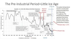
Figure 1. Yair Rosenthal’s temperature reconstruction of the 500-meter water in the Indonesian Throughflow.  To see image at full resolution click here.

Figure 1 shows a reconstructed temperature record from benthic foraminifera that live about 500 meters below the ocean surface in the Indonesian Throughflow. The reconstruction was made by Yair Rosenthal and colleagues and published in the journal Science. This is an ocean passage through the Indonesian islands that separate the Pacific from the Indian and Southern Oceans. The water temperatures there mostly reflect the temperature in the Northern and tropical Pacific, but they are influenced by the Indian and Southern Oceans to a smaller extent. I prefer this temperature proxy reconstruction to the various Greenland ice core reconstructions because it represents a much larger portion of the Northern Hemisphere climate system. That said, this reconstruction is similar to the Greenland ice core reconstructions in both shape and amplitude.

The Northern Hemisphere is where most people live, and it contains most long-term temperature proxies. Temperature proxies in the Southern Hemisphere are rare. Further, recent Southern Hemisphere temperature warming trends are much lower than in the Northern Hemisphere.

This reconstruction shows a drop in temperature of about 3°C from 4500BC to the depths of the Little Ice Age in 1750AD, Bo Vinther’s Greenland ice core temperature reconstruction also shows a three-degree drop, as shown in Figure 2. Attempts at hemispheric reconstructions, like Michael Mann’s hockey stick, always understate temperature variability due to averaging disparate temperature proxies and their inevitably inaccurate proxy radiometric dates.

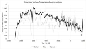
Figure 2. A plot of Greenland ice core reconstructions by Richard Alley, Bo Vinther, and Takuro Kobashi. Kobashi’s only goes back to 2000BC. Alley’s reconstruction, while more commonly seen, is uncorrected for elevation and is erratic during the very warm Holocene Climatic Optimum from 8000BC to 4500BC. Vinther’s is corrected for elevation changes and shows a prominent Holocene Climatic Optimum that is over three degrees warmer than the pre-industrial period. The references and more can be seen here and here.

So, it appears likely that Northern Hemisphere temperatures of the Holocene Climatic Optimum (roughly 9000BC to 4200BC) were more than three degrees warmer than those in the pre-industrial period, also known as the Little Ice Age. The IPCC 1750AD pre-industrial cutoff is shown with a vertical blue line in Figure 1. The present-day temperature at 500 meters, averaged from 2006 to 2016, is shown as a red box. The present-day data are from Viktor Gouretski at the University of Hamburg. The Rosenthal reconstruction displayed has a value every twenty years, the temperature error is about a third of a degree and the generally accepted temporal resolution is about plus or minus 50 years.

If we add 1.5 degrees to today’s temperature, we reach 9.2°C, this is roughly the same temperature in the Indonesian Throughflow, that was seen during the Roman Warm Period, labeled as RWP, or the temperature when Plato lived and taught. It is well over one-degree cooler than during the Holocene Climatic Optimum when human civilization and human agriculture were invented. We see no evidence in this reconstruction that 1.5, or even 2°C of warming were a problem in the past.

We also see no evidence that the pre-industrial period is a good standard global temperature. It was the coldest period in the entire Holocene. The Little Ice Age cold period did not occur everywhere in the world at the same time, but it was the closest our planet has been to a return to glacial conditions in the past 12,000 years. In Europe, Greenland, and North America, the coldest time was from about 1650 to 1750AD, coinciding with the Maunder Minimum, a period of low solar activity from 1645 to 1715. In the Rosenthal record the coldest time was about 1800 to 1815.

Cold spells frequently occurred during the pre-industrial period causing humanity many problems. Paul Homewood as well as Wolfgang Behringer’s excellent book, A Cultural History of Climate, and an article by Geoffrey Parker offer us a lot of historical examples. All over the world most glaciers reached their maximum Holocene extent during the Little Ice Age. In Chamonix, France they swallowed entire villages as they advanced.

There was no summer during 1675, and it was the second coldest summer in the past 600 years in North America according to proxy evidence. The winter of 1657-1658 was particularly brutal. Massachusetts Bay and the Delaware River both froze over, allowing people and deer to cross on the ice. The Baltic Sea froze so hard that horses and loaded wagons could cross from Gdansk, Poland to the Hel Peninsula over 10 miles north of the city. Yet, the following summer was excessively hot in Italy and Greece. In India the monsoon failed that year, resulting in a devastating famine.

Between 1660 and 1680, more typhoons struck southern China at Guangdong Province, than at any other time in recorded history. In 1666, a hailstorm hit England and some of the hailstones were a foot in circumference—softball size.

An enormously destructive hurricane hit the Caribbean Islands of Guadeloupe and Martinique in 1666 that resulted in 2,000 deaths and the destruction of a shore battery with walls 6 feet thick, as well as numerous ships.

Egypt in the 1670s had many very severe winters and people began to wear fur coats, something that had never happened in Egypt before. In the 1680s, the Sahel in Africa suffered a severe drought and Lake Chad reached the lowest level ever recorded.

The winter of 1691-1692 was very severe, starving wolves entered Vienna, Austria and attacked men and women on the streets. All the canals in Venice froze over and the mouth of the Nile River was choked with ice for a week. The cold of the 1690s caused a major famine in northern Europe and half the population of Finland died, as well as 15% of the population in Scotland. The Scottish famine was an important factor in its forced union with England. Mixed in with the cold years were occasional summers of intense heat and drought, such as the summers of 1693 and 1694 when the heat was unbearable in both England and Italy. Los Niños were more common during the Little Ice Age than now. Los Niños are nature’s way of expelling heat from the oceans to be radiated to space, this process can cause high atmospheric temperatures during the El Niño event itself, but the El Niño, ultimately cools the Earth once the atmospheric heat is radiated away. After cooling stops, Los Niños begin to decrease in frequency.

In 1715 a devastating hurricane struck the Bahamas and Florida killing between 1,000 and 2,000 people. That winter it was -20°C in Paris. There was a frost fair in London on the frozen Thames that year, with bonfires roasting oxen, carriages driven on the ice, and ice skating.

We have emphasized the worst portion of the Little Ice Age (1650-1715), but overall, it lasted from around 1300 to 1850. The first extraordinary cold weather spell of the LIA began in different places at different times, but in Europe, it began around 1310, with a series of very cold and wet winters that lasted until 1330. At first the crops, though poor, were adequate, but by 1315, the great famine began and was followed by the Black Death, from 1346-1352, which killed over one-third of Europe’s population.

European society had no concept of the accidental, someone was always to blame for catastrophe. It was either a person or group that caused it or sinned causing God to create the catastrophe. They did not believe nature acted alone. So, it was not long before Jews were blamed for the famines, cold, and floods. Thousands of them were killed. Then later, in the 1400s, it was witches, as illustrated by the 1486 woodcut shown in Figure 3. In the woodcut we see a witch using the jawbone of an ass to conjure up a hailstorm. Over 50,000 supposed witches were killed between 1500 and 1700.

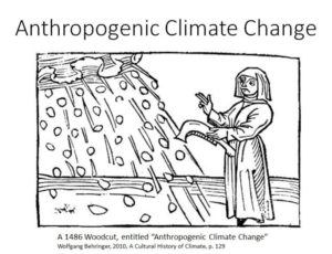
Figure 3. Anthropogenic Climate Change

The current “climate consensus” is not the first group in history to blame the weather on human activities. This is a recurring theme in human history. Figure 3 is from Behringer’s book, a bit more on his book can be seen here.

That is a brief introduction to the pre-industrial period. The IPCC’s “standard climate” against which our current global average temperatures are judged. The depths of the Little Ice Age coincide with the Maunder Grand Solar Minimum and the coldest part of the most recent Hallstatt-Bray cycle. There is always a climate rebound after Grand Solar Minimums and Hallstatt-Bray cold periods. The real question is why the Little Ice Age did not reach a full glacial? Not why did it warm afterward? I don’t know about you, but I think our current weather is better than the pre-industrial. Probably the next full glacial is already baked in and will start between 1,500 and 2,500 years from now. Our most serious climate change challenge is how do we adapt to that? Global warming is nothing in comparison.

Now we have defined and explained the terms used in the question put to Happer and Karoly, and their initial answers. Let’s examine their views in Figure 4. Karoly thinks that additional CO₂ emissions are dangerous because they will cause severe changes to the climate, especially global warming. We have just seen that the climate might have been worse during the pre-industrial period than it is today. Karoly does acknowledge that additional CO₂ will be beneficial to plants and crops, he just thinks climate change problems are worse than the benefits.

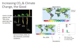
Figure 4. The good aspects of increasing CO₂ and global warming. To see image at full resolution click here.

Happer delves into the details of the benefits of more CO₂ for plant life. On the left of Figure 4, we see the result of a controlled experiment by Dippery, et al. (1995). Using the CO₂ concentration from the last glacial maximum, the plant grows very little in 14 days, at a CO₂ concentration of 350 ppm from around 1990, growth is robust. At a future concentration of 700 ppm much more growth is achieved. On the right we see the results of Zaichun Zhu’s study of the greening Earth from the journal Nature Climate Change.

The upper illustration is a map showing where greening is occurring using satellite data to estimate the change in the leaf area index (LAI) from 1982-2009. Zhu used three satellite datasets to do these estimates and they all show that the Earth has greened considerably. The upper map uses the Globmap dataset. Where it shows green, blue, or pink, there is more plant cover in 2009. Where it shows yellow or red, the area has browned, and has less plant cover. Most of the world is now much greener than in 1982.

Overall, Zhu reports that 21-46% of the global vegetated area is now greener and less than 4% is browner. His simulations show that 70% of the greening is due to additional CO₂. The lower map is a simulation of the greening only due to CO₂. The left red bar in the histogram is the observed greening, and the righthand bars show the modeled components of the increased greening, green is the CO₂ component, climate change or warming is shown in yellow, blue is additional nitrogen deposition, and purple is additional cultivated land. These results are from a multi-model ensemble mean abbreviated as “MMEM.”

Generally, observations, and modeling show that adding CO₂ to the atmosphere benefits plant life, which in turn makes our lives better.

Figure 5. CO₂ Coalition graph of increasing corn yields and CO₂ emissions.

Figure 5 is an interesting graph of global carbon emissions and corn yields from 1860 to 2020. The graph is by the CO₂ Coalition. The corn yields are from Bob Nelson at Purdue and the CO₂ data is from the Appalachian State University CO₂ database maintained by Gilfillan, et al. It shows the correlation between rising CO₂ levels and crop yields.

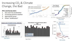
Figure 6. Increasing CO2 and global warming, the bad. To see image at full resolution click here.

The IPCC claim that global warming will cause sea level to rise quicker, more extreme weather, agricultural yields to fall, and will lower the ocean pH, the so-called ocean “acidification.” They project that these trends will cause problems in the future. But what does the data in Figure 6 show? NOAA’s sea level graph, top center, shows some acceleration in sea level, the period from 1880 to 1970 is very linear, with sea level increasing at five inches per century. From 1971 to 2022, the rate is 9 inches per century, an increase, but still not very scary. After all, the daily tidal range in the open ocean is two feet and much higher in many coastal areas. Right of the NOAA sea level data is a graph showing sea level rise since the last glacial maximum. It shows that sea level rise has been much higher in the past, especially prior to 5000BC during the Holocene Climatic Optimum when human civilization began.

Weather related disaster costs, as a percent of global GDP, have been decreasing rapidly for the past 30 years as shown by Roger Pielke Jr.’s histogram on the lower left of Figure 6. He has also plotted the total number of climate or weather-related disasters from the EM-DAT database since 2000, and the total number are also decreasing. This is not surprising; nights are warming faster than days and winters more than summers. In short, the weather is becoming milder with time, less extreme, not more.

Finally, as Bjorn Lomborg has shown in his 2020 paper, the number of climate and weather-related deaths has fallen dramatically since 1920, while non-climate-related deaths due to natural disasters have dropped much less, as shown on the lower right of Figure 6. In short, there is no evidence that sea level rise or extreme weather are problems today.

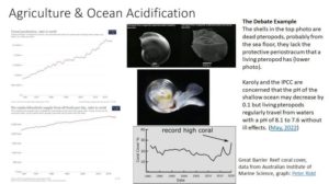
Figure 7. Crop yields and ocean acidification. To see image at full resolution click here.

Figure 7 examines the exchange between Happer and Karoly on ocean acidification and agricultural yield trends. The left graphs show the world-wide trends in cereal production (top graph) and in the number of food calories available per person (bottom graph) since 1961. Both are increasing in a nearly linear trend. In previous figures we saw that the correlation between increasing CO₂ emissions and corn yields since 1860, was striking; and Zhu estimated that 70% of increasing plant growth is due to increasing CO₂ and warmer temperatures. No sign of any problems here.

Ocean acidification is a misnomer. The ocean surface water pH is about 8.1, which is basic, not acidic. Areally, pH varies from about 8 to 8.25 depending mostly upon latitude, it is a bit lower in the tropics and a bit more basic at the poles. The pH typically decreases with water depth, proximity to land, and season, and can reach values as low as 6 (truly acidic) in rare natural environments. All shelled animals and fish have built in defenses that protect them from changing pH in this natural range. The decrease in pH since 1770, presumably due to increasing CO₂, is about 0.11, the highest change is in the Arctic, where pH has decreased 0.16. These are very tiny changes and fish, and shelled animals live through these sorts of changes every day.

The pH varies on the ocean surface from daytime to nighttime more than the average has changed since 1770. When CO₂ is absorbed by the ocean during the daytime it is rapidly taken up by phytoplankton for photosynthesis. At night, when the phytoplankton respire, the pH drops by about 0.7 units. Obviously, the fish in the water have no problem with this.

As shown on the right of Figure 7, some dead pteropods will corrode when they fall to the ocean floor. The ocean floor can be corrosive. This upper figure was presented in the debate as evidence that decreasing pH is dangerous to shelled animals. This is only true if the shelled animal is already dead. A living pteropod is shown below the dead ones and it is fine because it has a periostracum that adjusts the pH in the region where the living animal makes its shell. The periostracum can handle external pH values from well over 8.3 to 6 with ease. No pH values outside these ranges are projected.

As for the Australian Great Barrier Reef, the data shown in Figure 7 from the Australian Institute of Marine Science shows it now contains a record amount of coral. The reef is fine and not in danger.

The economic consequences of global warming and increasing CO₂ were only touched on in the debate, but we want to mention the work on climate change economics by Yale Professor William Nordhaus. Nordhaus won the Nobel Prize in Economics in 2018 for his work on climate change economics. The graphs in Figure 8 are from his Nobel Prize acceptance lecture, given in Sweden in 2018. His analysis of the IPCC estimated costs of global warming and the cost of reducing or eliminating fossil fuel CO₂ emissions shows that the optimum economic global warming path is the orange line identified with triangles in the left-hand graph. The Y axis is increasing global temperature in degrees C. His optimal path warms 4 degrees by 2130. The right-hand graph compares the cost of reducing fossil fuel use, in red, to future costs due to preventing warming, in green, as estimated by the IPCC. The optimal scenario is compared to a base case in which nothing is done, and cases where mitigating CO₂ emissions are done to keep warming below 2 and 1.5 degrees over the next 100 to 200 years.

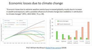
Figure 8. Professor William Nordhaus’s climate change economic analysis. To see image at full resolution click here.

Nordhaus chose an extreme global warming scenario, one that does not agree with observations, as we see in Figure 9. Thus, you are looking at an analysis of possibly inflated costs due to inflated projected warming. Nonetheless, it is clear we cannot afford to reduce fossil fuel use to limit warming to 1.5 to 2 degrees, the cost of abatement is simply too high.

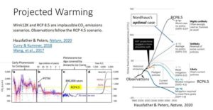
Figure 9. CO₂ emissions scenarios in context. To see image at full resolution click here.

On the right side of this slide, we see a realistic assessment of various IPCC CO₂ emissions scenarios. The summary is from an article in Nature in 2020 by Zeke Hausfather and Glen Peters, neither of these scientists are skeptics or “deniers.” They are very mainstream and are upset that the extreme and very unlikely RCP8.5, and the newer AR6 SSP3-7.0, scenarios are being portrayed in the media as “business as usual.” They both represent an “unlikely high-risk future” that has been discredited in the peer-reviewed literature.

Nordhaus’s optimal scenario is like the second from the top in Figure 9, labeled “Unlikely,” where temperatures reach 4°C by 2100 (Nordhaus, 2018, p. 452). Recent observations are well below this scenario and follow the RCP4.5 scenario. To provide some geological context, we show the RCP4.5 level of CO₂, in the year 2100, on a plot of CO₂ concentration for the past 500 million years. As you can see this level of CO₂ was exceeded between 50 and 20 million years ago around the PETM (the Paleocene-Eocene Thermal Maximum), when temperatures were probably ten degrees warmer than today. This was also the time when our ancestors. the primates, evolved and spread widely around the world. Primates, other mammals, new species of turtles, lizards, and many plants evolved and spread widely during this very nice, warm climate.

Conclusions

Is CO₂ good or bad? In summary, currently we have observed no negative effects from rising CO₂ or global warming. In fact, if anything, the world is better now than during the pre-industrial period. We have fewer weather and climate related problems, agricultural productivity is higher, and there are credible models that ascribe these improvements to rising levels of CO₂ and warmer weather.

The global economy is currently growing at about 3% per year, and nobody expects that growth rate to change much. At that rate, the economy will be 1,000% larger in 2100 than today. A 2% growth rate, the historical average, results in 478% growth in global GDP by 2100. The IPCC estimates that this will be reduced by 3% due to climate change, meaning we would see 464% growth, rather than 478%. The question is, will anyone notice? In the meantime, we will radically destroy our economy today, by eliminating fossil fuels, to save 14% growth in 2100. Is this smart? That is the question we need to ask ourselves.

Nordhaus claims that the optimal economic scenario leads to four degrees of global warming. Current realistic projections say we might see 2.5 to 3°C of warming in 2100. What is the fuss? More than 6000 years ago, temperatures were at least three degrees warmer than today in the Northern Hemisphere when civilization began. All Karoly and the IPCC have are ominous projections of future warming, with further projections of damages based them. None of their projections have been validated, and they have been invalidated by Ross McKitrick and John Christy in two recent critical papers, published in 2018 and 2020.

Calm down folks, there is nothing to worry about.

The event was a luncheon talk, that sold out completely at $70 a plate. Lots of applause and there were several questions afterward, all polite. The hosts put on a book signing afterward for me and I sold every book I brought and have pre-paid orders for several more. A good day.