This post is a result of an online conversation with Dr. Leif Svalgaard, a research physicist at Stanford University. Leif knows a great deal about the Sun and solar variability and can explain it clearly. Our disagreement is over whether long-term solar variations could be large enough to affect Earth’s climate more than changes due to humans – or not. Thus, we are arguing about the relative magnitudes of two sources of radiative forcing (RF) that are not known accurately. The IPCC estimates that the total RF, due to humans, since 1750, is 2.3 W/m² (IPCC, 2013, p. 696). This number is unverifiable and likely exaggerated, but we can accept it for the sake of this argument.

I’ve written on this topic before here. This post is an update and will not cover the same ground. Some readers will want to read the first post before this one.

The question becomes, could the Sun change enough to deliver more than half of 2.3 W/m², or 1.15 W/m², of power to Earth’s surface since 1750? The IPCC and Svalgaard believe that, since 1750, the change in solar output nets to zero, or close to it:

“The point is that solar activity has had no measurable effect on climate over the past several centuries.” Dr. Svalgaard, July 7, 2021.

Svalgaard then suggests I read an article by Mike Lockwood and William Ball in Proceedings A of the Royal Society (Lockwood & Ball, 2020). The article is an excellent overview of the debate over long-term changes in solar RF on Earth. Because Earth is a rotating sphere and half of it is in darkness, a change of one W/m² in solar output only causes a 0.25 W/m² change in solar RF at the top of the atmosphere. Thus, to achieve the aforementioned 1.15 W/m² change in RF at the surface, taking Earth’s likely albedo into account, the Sun’s output needs to increase 6 W/m² since 1750. To account for all the warming, since 1750, it must increase 12 W/m², a 0.9% increase in solar output.

Most writers only consider “TSI” or Total Solar Irradiance, when they consider solar RF delivered to Earth, but the Sun varies in other ways that influence our climate independently of the Sun’s direct total radiation output. For example, the Sun’s UV (ultraviolet) radiation varies more than the total and the Sun’s magnetic field strength varies significantly at Earth’s orbit, as well as the power of the so-called “solar wind” of charged particles (Haigh, 2011). TSI variation is not the only way the Sun can influence our climate, but it is something we can measure. Unfortunately, some scientists often only focus on those things they can measure and consider unmeasurable quantities to be “insignificant,” whether they are or not. We will limit this post to TSI variability but be aware it is only part of the story.

Large scale changes in solar output are determined by changes in the solar magnetic field and these changes are understood reasonably well. Svalgaard often points this out and I have no problem with his reasoning along these lines. Less well understood are the contributions to solar variability made by the quiet regions of the Sun. The quiet regions, or “Q regions,” are the featureless portions of the solar surface or photosphere. These are areas without sunspots or other visible magnetic features. As Lockwood and Ball remind us, there are little data on variations in the quiet solar regions.

TSI is a blunt instrument, it is the total electromagnetic power, integrated over all wavelengths, that reaches the average Earth orbit. Most of this power is generated in Q regions in flux tubes too small for us to detect, but very important because they are so numerous. Sunspots are much larger flux tubes, as are the bright faculae that surround them, so large we can easily see them. Thus, what Svalgaard and many other astrophysicists believe, is that by keeping track of the larger sunspots and sunspot-related features in the Sun’s photosphere, they can detect all significant solar variability. The reasoning is, we cannot measure any changes in the Q region, so they must be insignificant.

As already mentioned, for the Sun to be the dominant (that is >50%) cause of recent warming, the Sun would have to increase its output about 6 W/m² since 1750, or 0.02 W/m²/yr on average. The IPCC and Svalgaard prefer the PMOD TSI composite, but there are other TSI composites, see here for a discussion. Lockwood provides an interesting plot of satellite measurements of TSI and alternative composites versus the PMOD TSI model composite.

His plot is shown in Figure 1. The yellow dots (CCv01) are the community composite, which is very similar to PMOD. The mauve circles are the RMIB composite. The RMIB (also abbreviated IRMB) composite is plotted in our earlier post.

Figure 1. A comparison of various satellite TSI measurements and two other TSI composites to the PMOD TSI model. Source: (Lockwood & Ball, 2020). All points are means over Carrington solar rotation periods, roughly 27 days. The lines show the trends versus the PMOD trend. The trends vary from 0.0261 W/m2/yr to -0.0255 W/m2/yr for a total difference of 0.052 W/m2/yr.

The Sun is complex, and it is not solid, thus the rate of solar rotation varies by latitude, it rotates faster at the equator and slower near the poles. The Solar rotation rate is usually given as ~27.3 days, which is called the Carrington rotation, often abbreviated as “CR.” In Figure 1, TSI satellite measurements are plotted as CR averages, and differences from the PMOD model composite are shown, as well as the trend of the differences. Six satellite instruments are plotted and the difference in rate from the lowest trend (ACRIM-3) to the highest trend (TIM) is 0.052 W/m²/year. All these measurements and composites are peer-reviewed and reasonable; thus, the different trends can be considered an estimate of TSI uncertainty. We cannot measure the long-term change in total solar output accurately enough to preclude the necessary change of 0.02 W/m²/yr.

A difference of 0.052 W/m²/year is a change of 13.6 W/m² since 1750. This is more than the total anthropogenic change in forcing (12 W/m²) computed by the IPCC since the beginning of the industrialized era. The readers of our earlier post will know that using NOAA’s estimates of the error in our solar output measurements result in uncertainties as high as 34 to 47 W/m² since 1750. We simply do not know enough about the long-term variability of the Sun to preclude it as a cause of current warming.

Various recent reconstructions of TSI to 1600 AD are shown in Figure 2, also from Lockwood and Ball.

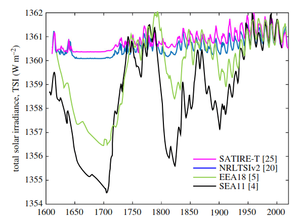
Figure 2. Four recent TSI reconstructions. The two invariant reconstructions (SATIRE and NRLTSI) are based on active portions of the Sun only, that is sunspots and related features. The more active reconstructions (EEA and SEA) attempt to incorporate Q region variability. Source: (Lockwood & Ball, 2020)

Figure 2 shows a range of recent TSI reconstructions. The SATIRE (Wu, Krivova, Solanki, & Usoskin, 2018) and NRLTSI (Coddington, et al., 2019) reconstructions are suspiciously flat during the period of the Maunder Minimum (1645-1715) when there were very few sunspots and temperatures on Earth were very cold. This was the coldest period of the Little Ice Age, as described by Wolfgang Behringer (Behringer, 2010) and here. Behringer reports that during this period the canals of Venice froze, and heavy goods could be transported across them in wagons. Due to the cold, the related malnutrition, and epidemics, the worst mortality crisis in European history occurred in the early 1600s. Witches and Jews were blamed for the cold and thousands were executed, often they were burned alive. The killings reached their peak in the early 1600s. Behringer comments that the belief that witches and Jews caused the global cooling, was the medieval equivalent of “Anthropogenic Climate Change,” see figure 4 in this earlier post.

Records of similar crises exist for China, Indonesia, Thailand, and the Philippines. Glaciers advanced around the world at this time, and according to Bray’s classic 1968 paper, more worldwide maximum glacial advances occurred from 1587 to 1798 than in any other period he studied (Bray, 1968).

The year 1816 is often known as the “year without a summer” (Behringer, 2010, p. 163). Usually, this is blamed on the eruption of Mt. Tambora in 1815, but it also coincides with a steep decrease in TSI according to both the EEA and SEA reconstructions in Figure 2. Likewise, the well documented steep global warming from 1910 to 1944 is visible on both of these TSI reconstructions. Historical records are not quantitative data, but they are consistent with the more active solar reconstructions, and they occur before fossil fuel CO₂ emissions were significant.

The SATIRE and NRLTSI reconstructions assume that the Q region is constant over the period and are based largely on sunspot records. Egorova, et al. [EEA18 or (Egorova, et al., 2018)] and Shapiro, et al. [SEA11 or (Shapiro, et al., 2011)] incorporate estimates of Q region variablity and the result is a range of TSI over the period as shown in Figure 2 of 1354.5 to 1362 (7.5 W/m²). This range is over half the total needed to account for all the warming since 1750, the aforementioned 12 W/m².

Lockwood, et al., Egorova, et al., and Shapiro, et al. all emphasize that there is no agreed modern TSI composite of the satellite measurements to date, this is illustrated in Figure 1. The intensity of solar radiation in space is so severe it begins affecting the instruments nearly as soon as they are first pointed toward the Sun. As a result, both the magnitude of TSI and its long-term trend is unclear.

We can see the problem. There is no agreed record of satellite era total solar variability. Sunspots are only a record of the variability in the more active portions of the Sun, and the Q region variability has never been observed or measured. Models of the Q region are speculative. This is an important issue because solar variability is an obvious possible cause of recent global warming, and the IPCC wants to claim it is constant. They have no evidence for this, but, on the other hand, the evidence it is more active in the Q region is indirect and weak.

Egorova, et al., 2018, is the most recent paper to present a model of TSI that includes Q region variablity, so we will focus on it. It is notable that A. I. Shapiro, the senior author of Shapiro, et al., 2011, is a co-author of Egorova’s paper. Dr. Egorova works at the Physikalisch-Meteorologisches Observatorium Davos, the home of the PMOD TSI reconstruction. Like all TSI reconstructions, Egorova models the active regions of the Sun with sunspot data, but she models the Q region differently. The problem she, Shapiro, and the other more active Sun reconstruction researchers have, is the Sun is now bright and it has never been observed with modern instruments in a quiet period, like the Maunder Minimum.

Like Shapiro, et al., Egorova assumes that variations in Q region solar output vary due to the level of solar magnetic activity in the preceding decades. They vary TSI linearly between the current solar maximum and the lowest estimated magnetic activity of the Sun. They use the solar modulation potential, or ф, as a proxy for solar magnetic activity. The solar modulation potential is strongly related to the open solar flux that shields Earth from galactic cosmic rays. Instrumental values of ф are available to 1936 (Usoskin, Bazilevskaya, & Kovaltsov) and can be extended into the past using a ¹⁰Be proxy that is sensitive to the number of galactic cosmic rays that strike Earth. More on ¹⁰Be and the Sun can be seen here.

Conclusions

None of the TSI reconstructions plotted in Figure 2 are well supported. The more active regions of the Sun can be modeled using sunspot records reasonably accurately, but this ignores most of the Sun. Our measurements of TSI, from satellites, conflict with one another and all instrumental TSI composites are in doubt due to instrument problems and the dubious “daisy-chain” composites.

We are currently in a solar maximum and have no measurements of the Sun in a solar minimum, so all reconstructions of the Sun in a solar minimum are speculative extrapolations. The SATIRE and NRLTSI reconstructions dodge this issue by assuming that the Q region of the Sun is constant and never changes. Thus, they have a very unrealistic flat spot during the historically well documented Maunder Minimum. Egorova and Shapiro try to extrapolate a value into the Maunder Minimum using proxies to estimate ф. Since ф is correlated closely to the open solar flux, this is reasonable, but still speculative.

Historical data supports the more active reconstructions since they correlate to historical climatic events. The records of glacier advances during the Little Ice Age are also very supportive. Finally, the variability of other Sun-like stars suggests our Sun is much more variable than assumed in the SATIRE and NRLTSI reconstructions as shown in the following figure from Judge, et al. 2020.

Figure 3. The blue is the Shapiro, 2011 reconstruction, rescaled. The two red objects show observed variability in Sun-like stars elsewhere in our galaxy. The rate of change indicated, in red, on the left, is compatible with several stars studied by Judge, et al. and the one on the right is compatible with half of the stars in their study. Source: (Judge, Egeland, & Henry, 2020).

The jury is still out on this issue and will be until we can improve and lengthen our instrumental records of solar activity. This debate, like the debate over climate sensitivity, is the result of inadequate measurements of the critical variables. Measurement error swamps the differences in the two hypotheses.

This article appeared on the Watts Up With That? website at https://wattsupwiththat.com/2021/07/23/can-we-predict-long-term-solar-variability/