Investigating the leaf area index changes in response to climate change (case study: Kasilian catchment, Iran)
Abstract
Introduction
Case study
Materials and methods
BIOME-BGC model
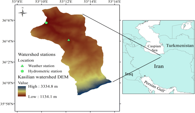
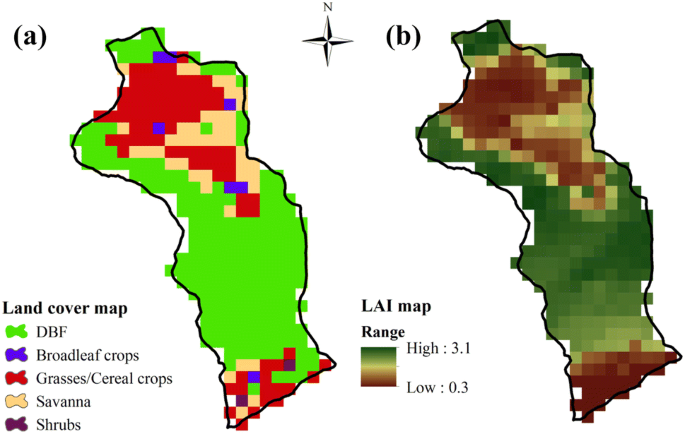
BIOME-BGC is a biogeochemical model which simulates main physiological processes such as photosynthesis, evapotranspiration, respiration, and decomposition within the terrestrial ecosystems [39, 51]. The latest version of this model is BIOME-BGC version 4.2, which can simulate several vegetation indices such as NPP, GPP, and LAI for 7 vegetation cover types such as the evergreen needle leaf forest (ENF), evergreen broadleaf forest (EBF), deciduous needle leaf forest (DNF), deciduous broadleaf forest (DBF), shrubs, C3 and C4 grasses, based on temporal scales of daily, monthly, and annual. BIOME-BGC model calculates LAI by multiplying carbon allocated to leaves times the specific leaf area. To simulate LAI using BIOME-BGC model with high spatial resolution, high-resolution land cover map and LAI values are needed. The only available land cover map in Kasilian catchment was related to the year 1995 and has a low spatial resolution of 2 km, while we needed a vegetation map with a higher spatial resolution at the beginning of the study period (2004). Moreover, there were no available field-LAI measurements for the Kasilian catchment. To address these restrictions, MODIS land cover product named as MODIS MCD12Q1 [9] and MODIS LAI product named as MODIS MOD15A2H [32] which have the same spatial resolution (500 m) were used in this study. Using MODIS products enabled us to develop gridded BIOME-BGC with a spatial resolution of 500 m within Kasilian catchment, and consequently, 319 pixels were created over Kasilian catchment area. The ecosystem process modeling using BIOME-BGC model includes two steps: In the first step, the model was run in a spin-up mode. Spin-up run is a common step for ecosystem models to ensure that it achieves stable ecosystem conditions in the desired site [52]. After achieving an equilibrium state, the model was run in normal mode. At this step, BIOME-BGC simulates carbon, nitrogen, and water cycles in the components of the plant and soil. BIOME-BGC model requires three main categories of information, including climatic data, environmental information, and eco-physiological parameters (Table 1). The climatic data in each pixel were simulated using the weather simulator of BIOME-BGC model called “Mountain Climate Simulator” (MT-CLIM model) [50]. Other environmental information of each pixel, including elevation, slope, slope’s direction, and soil texture information (silt, clay, and sand), was obtained from a digital elevation model (DEM) and basin’s soil map, respectively. These environmental data were re-gridded to a 500 m spatial resolution to enter the BIOME-BGC model.Evaluation of BIOME-BGC model
To evaluate the gridded BIOME-BGC model accuracy, BIOME-BGC monthly LAI output was compared against monthly MODIS-derived LAI using three statistical criteria including R2 (coefficient of determination), RMSE (root mean square error), and percent error (PE) shown in Eqs. (1), (2), and (3), respectively, where X: the monthly MODIS LAI, Y: the monthly BIOME-BGC LAI, and N: the total number of monthly MODIS LAI (N = 120). Low quantities of RMSE and PE and high quantities of the coefficient of determination (R2) represent the acceptable accuracy of BIOME-BGC model.Climate change projections
Climate models
At present, AOGCMs (atmosphere-ocean general circulation models) are the most credible climate simulators that have been used in ecosystem studies [35, 47]. In this study, climate projections from the average of 9 AOGCMs, used in the Intergovernmental Panel on Climate Change (IPCC) Fifth Assessment Report (AR5), are applied to assess potential climate change impacts on LAI (Table 3). RCP2.6 and RCP8.5 are emission scenarios chosen in this study [30, 54]. These scenarios were used because RCP2.6 and RCP8.5 scenarios cover the minimum and maximum conditions of the emission scenarios in the future, respectively.Preparing climate model scenarios
To create a climate change scenario for each AOGCM, the delta method was used (Eqs. 4, 5, and 6).LARS-WG model
To introduce daily climate data to the BIOME-BGC model in the future period (2020–2039) under the climate change scenarios, a weather generator model called LARS-WG was used [2]. LARS-WG model (version 5.5) is a stochastic weather generator which is useful for generating the daily time series of maximum and minimum temperatures (degrees Celsius) and precipitation (millimeters) in a climate station under current and future climate conditions [36, 41]. The modeling processes using LARS-WG model are composed of three main steps, including calibration, evaluation, and generation of meteorological data for the future. In the calibration step, the probabilistic distribution parameters of the observed daily climate variable (1986–2005), including daily maximum and minimum temperatures and precipitation, were analyzed and computed. In the second step, the ability of the LARS-WG model to simulate daily climate data during the baseline period (1986–2005) was evaluated by comparing observed and simulated climate data. In the third step, by introducing the ensemble average climate change scenario under RCP2.6 and RCP8.5 emission scenarios created by Eqs. (7), (8), and (9), daily climate data for 2020–2039 were generated under future climate conditions.Results and discussion
Evaluation results of BIOME-BGC model
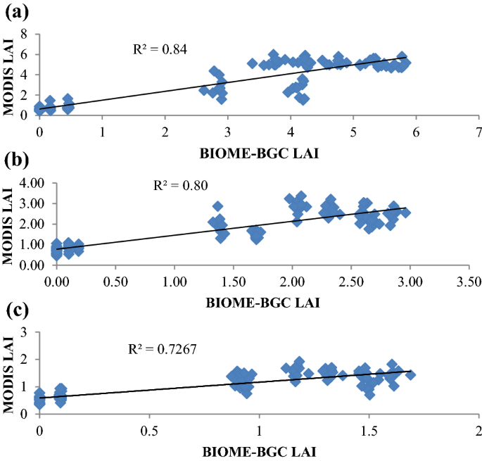
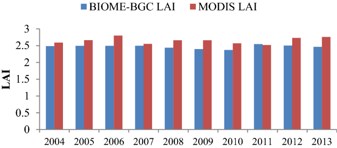
The monthly LAI values were simulated by BIOME-BGC in 319 pixels separately over the Kasilian catchment. The amount of calculated R2 is greater than or equal to 0.7 (R2 ≥ 0.7) in all pixels which demonstrate that monthly MODIS LAI and BIOME-BGC LAI were in good agreement. As an example, the scatterplot of the monthly MODIS LAI and BIOME-BGC LAI for three pixels including deciduous broadleaf forest (DBF), shrubs, and C3 grasses is shown in Fig. 3a, b, c, respectively. Although the R2 values indicate an acceptable correlation between monthly MODIS LAI and BIOME-BGC LAI, the values of percentage error (PE) and RMSE show a small amount of error between these two LAI time series. The PE and RMSE values in all pixels were less than or equal to 30% and 0.9, respectively. This error is resulted from the inability of BIOME-BGC model to simulate the rapid growth of plants in the early part of the growing season. Furthermore, the comparison of the annual mean values of the MODIS LAI and BIOME-BGC LAI showed a slight discrepancy from 2004 to 2013 (Fig. 4). Figure 4 also demonstrates that BIOME-BGC model simulated the annual mean LAI values with high accuracy in all years.Changes in climate variables and CO2 level
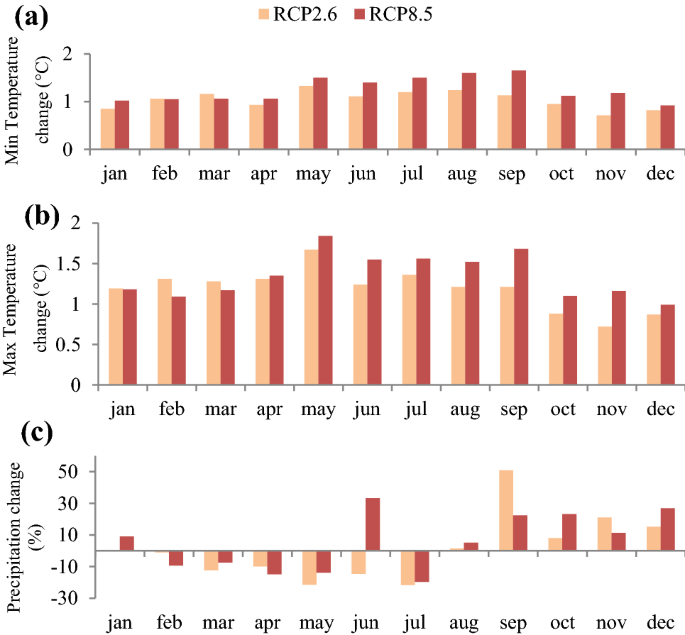
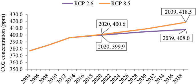
Monthly changes of minimum temperature, maximum temperature, and precipitation in the future period (2020–2039) relative to the baseline period (1986–2005), calculated based on Eqs. (7), (8), and (9), are shown in Fig. 5a, b, c, respectively. The results showed that minimum and maximum temperature would increase under both scenarios (RCP2.6 and RCP8.5) in all months. Under both scenarios, minimum and maximum temperatures are expected to increase more in May, June, July, August, and September compared to other months in the future period. It is also projected that minimum and maximum temperatures under the RCP8.5 scenario will see a higher increase compared to the RCP2.6 scenario in all months, with an exception in February and March.Evaluation of the LARS-WG model
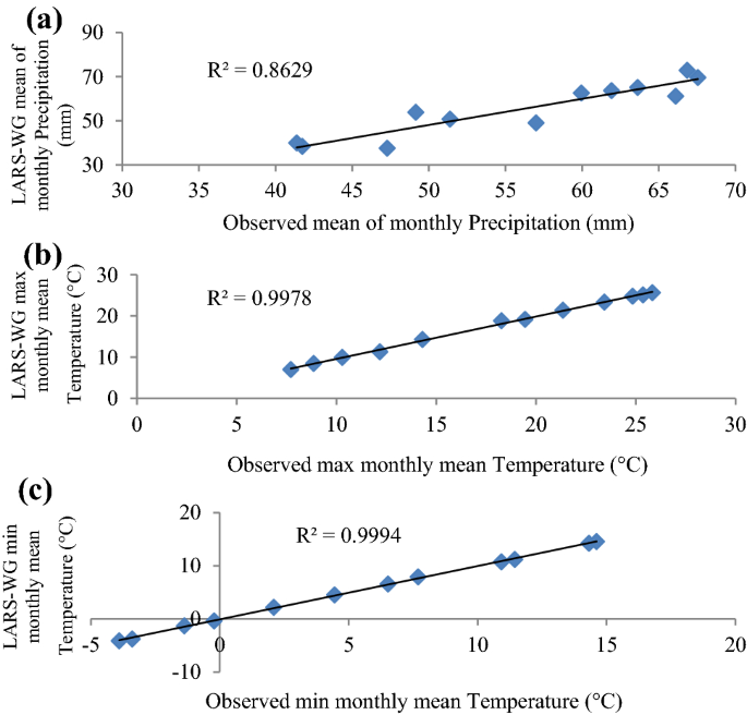
Figure 7a, b, c shows scatterplots between monthly mean values of minimum temperature, maximum temperature, and precipitation simulated by the LARS-WG model and observed data at “Darzikola” climatology station located in the Kasilian catchment during the baseline period (1986–2005). The high value of R2 between observed and simulated monthly mean minimum temperature, maximum temperature, and precipitation indicates that LARS-WG model regenerates climate variables with high accuracy at “Darzikola” climatology station. R2 value for monthly mean minimum and the maximum temperature is more than 0.99, and for monthly mean precipitation it is about 0.86. It represents that simulated monthly mean precipitation values have a relatively lower accuracy compared to simulated monthly mean minimum and maximum temperature.LAI changes under climate change
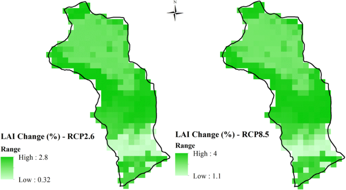
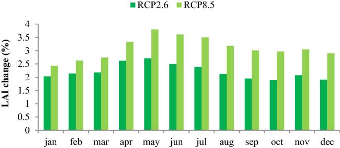
By introducing daily climate series generated by the LARS-WG model and annual level of CO2 derived from IPCC website (www.IPCC-data.org) to BIOME-BGC model, daily LAI series were estimated under RCP2.6 and RCP8.5 in the future period (2020–2039) in all pixels. Figure 8 shows percentage changes in monthly LAI in all pixels in response to changes in climate variables of temperature, precipitation and carbon dioxide concentration (ppm) under the RCP2.6 and RCP8.5 scenarios during the future period (2020–2039) compared to the study period (2004–2013).Conclusion
References
- 1.
Baret F, Hagolle O, Geiger B, Bicheron P, Miras B, Huc M, Berthelot B, Niño F, Weiss M, Samain O, Roujean JL (2007) LAI, fAPAR and fCover CYCLOPES global products derived from VEGETATION: part 1: principles of the algorithm. Remote Sens Environ 110:275–286
- 2.
Chen H, Guo J, Zhang Z, Xu CY (2013) Prediction of temperature and precipitation in Sudan and South Sudan by using LARS-WG in future. Theor Appl Climatol 113:363–375
- 3.
Chen JM, Black TA (1992) Defining leaf area index for non-flat leaves. Plant Cell Environ 15:421–429
- 4.
Collier MA, Jeffrey SJ, Rotstayn LD,Wong KK, Dravitzki SM, Moseneder C, Hamalainen C, Syktus JI, Suppiah R, Antony J, El Zein A, Artif M (2011) The CSIRO-Mk3.6.0 Atmosphere–Ocean GCM: participation in CMIP5 and data publication. In: International congress on modelling and simulation—MODSIM 2011, The 19th international congress on modelling and simulation (MODSIM2011) was held at the Perth Convention and Exhibition Centre in Perth, Perth, Western Australia, 12–16 December 2011
- 5.
Davoodi E, Ghasemieh H, Batelaan O, Abdollahi K (2017) Spatial-temporal simulation of LAI on basis of rainfall and growing degree days. Remote Sens 9:1207. https://doi.org/10.3390/rs9121207
- 6.
Dong T, Liu J, Qian B, Zhao T, Jing Q, Geng X, Shang J (2016) Estimating winter wheat biomass by assimilating leaf area index derived from fusion of Landsat-8 and MODIS data. Int J Appl Earth Obs Geoinf 49:63–74
- 7.
Donohue RJ, Roderick ML, McVicar TR (2006) On the importance of including vegetation dynamics in Budyko? s hydrological model. Hydrol Earth Syst Sci Discuss 3:1517–1551
- 8.
Fang H, Wei S, Liang S (2012) Validation of MODIS and CYCLOPES LAI products using global field measurement data. Remote Sens Environ 119:43–54
- 9.
Friedl MA, Sulla-Menashe D, Tan B, Schneider A, Ramankutty N, Sibley A, Huang X (2010) MODIS collection 5 global land cover: algorithm refinements and characterization of new datasets. Remote Sens Environ 114:168–182
- 10.
Ganguly S, Samanta A, Schull MA, Shabanov NV, Milesi C, Nemani RR, Gao F, Masuka E, Myneni R, Tan B, Nightingale J (2008) An algorithm to produce temporally and spatially continuous MODIS-LAI time series. IEEE Geosci Remote Sens Lett 1:1545–1598
- 11.
Gholami V, Jokar E, Azodi M, Zabardast HA, Bashirgonbad M (2009) The influence of anthropogenic activities on intensifying runoff generation and flood hazard in Kasilian watershed. J Appl Sci 9:3723–3730
- 12.
Gholzom EH, Gholami V (2012) A comparison between natural forests and reforested lands in terms of runoff generation potential and hydrologic response (case study: kasilian watershed). Soil Water Res 7:166–173
- 13.
Gigante V, Iacobellis V, Manfreda S, Milell P, Portoghese I (2009) Influences of Leaf Area Index estimations on water balance modeling in a Mediterranean semi-arid basin. Nat Hazards Earth Syst 9:979–991
- 14.
Giorgetta MA, Jungclaus J, Reick CH, Legutke S, Bader J, Böttinger M, Brovkin V, Crueger T, Esch M, Fieg K, Glushak K (2013) Climate and carbon cycle changes from 1850 to 2100 in MPI-ESM simulations for the Coupled Model Intercomparison Project phase 5. J Adv Model Earth Syst 5:572–597
- 15.
Hardwick SR, Toumi R, Pfeifer M, Turner EC, Nilus R, Ewers RM (2015) The relationship between leaf area index and microclimate in tropical forest and oil palm plantation: forest disturbance drives changes in microclimate. Agric For Meteorol 201:187–195
- 16.
Hao L, Pan C, Liu P, Zhou D, Zhang L, Xiong Z, Sun G (2016) Detection of the coupling between vegetation leaf area and climate in a multifunctional watershed, Northwestern China. Remote Sens 81:1032. https://doi.org/10.3390/rs8121032
- 17.
Hazeleger W, Severijns C, Semmler T, Ştefănescu S, Yang S, Wang X, Wyser K, Dutra E, Baldasano JM, Bintanja R, Bougeault P (2010) EC-Earth: a seamless earth-system prediction approach in action. Bull Am Meteorol Soc 91:1357–1364
- 18.
Idso SB (1988) Three phases of plant response to atmospheric CO2 enrichment. Plant Physiol 87:5–7
- 19.
Jones PD, Hulme M (1996) Calculating regional climatic time series for temperature and precipitation: methods and illustrations. Int J Climatol 16:361–377
- 20.
Kang S, Running SW, Kimball JS, Fagre DB, Michaelis A, Peterson DL, Hong S (2014) Effects of spatial and temporal climatic variability on terrestrial carbon and water fluxes in the Pacific Northwest, USA. Environ Model Softw 51:228–239
- 21.
Khaleghi MR (2017) The influence of deforestation and anthropogenic activities on runoff generation. J For Sci 63:1–9
- 22.
Kim JB, Monier E, Sohngen B, Pitts GS, Drapek R, McFarland J, Ohrel S, Cole J (2017) Assessing climate change impacts, benefits of mitigation, and uncertainties on major global forest regions under multiple socioeconomic and emissions scenarios. Environ Res Lett 12:045001. https://doi.org/10.1088/1748-9326/aa63fc
- 23.
Kimball BA, Idso SB (1983) Increasing atmospheric CO2: effects on crop yield, water use and climate. Agric Water Manag 7:55–72
- 24.
Krishnaswamy J, John R, Joseph S (2014) Consistent response of vegetation dynamics to recent climate change in tropical mountain regions. Glob Change Biol 20:203–215
- 25.
Krinner G, Viovy N, de Noblet-Ducoudré N, Ogée J, Polcher J, Friedlingstein P, Ciais P, Sitch S, Prentice IC (2005) A dynamic global vegetation model for studies of the coupled atmosphere-biosphere system. Glob Biogeochem Cycles. https://doi.org/10.1029/2003GB002199
- 26.
Kross A, Lapen DR, McNarin H, Sunohara M, Champagne C, Wilkes G (2015) Satellite and in situ derived corn and soybean biomass and leaf area index: response to controlled tile drainage under varying weather conditions. Agric Water Manag 160:118–131
- 27.
Mahowald N, Lo F, Zheng Y, Harrison L, Funk C, Lombardozzi D, Goodale C (2016) Projections of leaf area index in earth system models. Earth Syst Dyn 7:211–229
- 28.
Manea A, Leishman MR (2014) Leaf area index drives soil water availability and extreme drought-related mortality under elevated CO2 in a temperate grassland model system. PLoS ONE 9:91046. https://doi.org/10.1371/journal.pone.0091046
- 29.
Marsh DR, Mills MJ, Kinnison DE, Lamarque JF, Calvo N, Polvani LM (2013) Climate change from 1850 to 2005 simulated in CESM1 (WACCM). J Clim 26:7372–7391
- 30.
Moss RH, Edmonds JA, Hibbard KA, Manning MR, Rose SK, Van Vuuren DP, Carter TR, Emori S, Kainuma M, Kram T, Meehl GA (2010) The next generation of scenarios for climate change research and assessment. Nature 463:747. https://doi.org/10.1038/nature08823
- 31.
Myneni RB, Hoffman S, Knyazikhin Y, Privette JL, Glassy J, Tian Y, Wang Y, Song X, Zhang Y, Smith GR, Lotsch A, Friedl M, Morisette JT, Votava P, Nemani RR, Running SW (2002) Global products of leaf area index and fraction absorbed PAR from year one of MODIS data. Remote Sens Environ 83:214–231
- 32.
Myneni R, Knyazikhin Y, Park T (2015) MOD15A2H MODIS/Terra Leaf Area Index/FPAR 8-Day L4 Global 500 m SIN Grid V006 [Data set]. NASA EOSDIS Land Processes DAAC, https://doi.org/10.5067/modis/mod15a2h.006
- 33.
Nielsen DC, Miceli-Garcia JJ, Lyon DJ (2012) Canopy cover and leaf area index relationships for wheat, triticale, and corn. Agron J 104:1569–1573
- 34.
Piao S, Yin G, Tan J, Cheng L, Huang M, Li Y, Liu R, Mao J, Myneni RB, Peng S, Poulter B (2015) Detection and attribution of vegetation greening trend in China over the last 30 years. Glob Change Biol 21:1601–1609
- 35.
Pourmokhtarian A, Driscoll CT, Campbell JL, Hayhoe K, Stoner AM, Adams MB, Burns D, Fernandez I, Mitchell MJ, Shanley JB (2017) Modeled ecohydrological responses to climate change at seven small watersheds in the northeastern United States. Glob Change Biol 23:840–856
- 36.
Racsko P, Szeidl L, Semenov M (1991) A serial approach to local stochastic weather models. Ecol Model 57:27–41
- 37.
Ramezani MR, Massah Bavani AR, Jafari M, Binesh A (2017) Evaluating gridded BIOME-BGC for simulating LAI at Kasilian watershed-Iran. Geol Ecol Landsc 1:225–231
- 38.
Ran L, Pleim J, Gilliam R, Hogrefe C, Binkowski F, Band L (2016) Application and evaluation of MODIS LAI, FPAR, and Albedo products in the WRF/CMAQ System. In: Steyn DG, Chaumerliac N (eds) Air pollution modeling and its Application XXIV. Springer, Berlin, pp 619–624
- 39.
Running SW, Hunt ER (1993) Generalization of a forest ecosystem process model for other biomes, BIOME-BGC, and an application for global-scale models. In: Ehleringer JR, Field CB (eds) Scaling physiological processes: leaf to globe. Academic Press, San Diego, pp 141–158
- 40.
Running SW, Nemani RR (1991) Regional hydrologic and carbon balance responses of forests resulting from potential climate change. Clim Change 19:349–368
- 41.
Semenov MA, Brooks RJ, Barrow EM, Richardson CW (1998) Comparison of the WGEN and LARS-WG stochastic weather generators for diverse climates. Clim Res 10:95–107
- 42.
Schmidt GA, Kelley M, Nazarenko L, Ruedy R, Russell GL, Aleinov I, Bauer M, Bauer SE, Bhat MK, Bleck R, Canuto V (2014) Configuration and assessment of the GISS ModelE2 contributions to the CMIP5 archive. J Adv Model Earth Syst 6:141–184
- 43.
Sitch S, Smith B, Prentice IC, Arneth A, Bondeau A, Cramer W, Thonicke K (2003) Evaluation of ecosystem dynamics, plant geography and terrestrial carbon cycling in the LPJ dynamic global vegetation model. Glob Change Biol 9:161–185
- 44.
Srebin PS, Ahl DE, Gower ST (2013) Spatial and temporal validation of the MODIS LAI and FPAR products across a boreal forest wildfire chronosequence. Remote Sens Environ 133:71–84
- 45.
Stenberg P (1996) Correcting LAI-2000 estimates for the clumping of needles in shoots of conifers. Agric For Meteorol 79:1–8
- 46.
Stocker TF, Qin D, Plattner GK, Tignor M, Allen SK, Boschung J, Nauels A, Xia Y, Bex V, Midgley PM (2013) IPCC climate change 2013: the physical science basis, contribution of working group I to the fifth assessment report of the intergovernmental panel on climate change. Cambridge University Press, Cambridge
- 47.
Sun S, Sun G, Cohen E, McNulty SG, Caldwell PV, Duan K, Zhang Y (2016) Projecting water yield and ecosystem productivity across the United States by linking an ecohydrological model to WRF dynamically downscaled climate data. Hydrol Earth Syst Sci 20:935–952
- 48.
Tesemma ZK, Wei Y, Peel MC, Western AW (2015) The effect of year-to-year variability of leaf area index on Variable Infiltration Capacity model performance and simulation of runoff. Adv Water Resour 83:310–322
- 49.
Tesemma ZK, Wei Y, Western AW, Peel MC (2014) Leaf area index variation for crop, pasture, and tree in response to climatic variation in the Goulburn-Broken catchment, Australia. J Hydrometeorol 15:1592–1606
- 50.
Thornton PE, Hasenauer H, White MA (2000) Simultaneous estimation of daily solar radiation and humidity from observed temperature and precipitation: an application over complex terrain in Austria. Agric For Meteorol 104:255–271
- 51.
Thornton PE, Law BE, Gholz HL, Clark KL, Falge E, Ellsworth DS, Chen J (2002) Modeling and measuring the effects of disturbance history and climate on carbon and water budgets in evergreen needleleaf forests. Agric For Meteorol 113:185–222
- 52.
Thornton PE, Rosenbloom NA (2005) Ecosystem model spin-up: estimating steady state conditions in a coupled terrestrial carbon and nitrogen cycle model. Ecol Model 189:25–48
- 53.
Trombetta A, Lac obellis V, Tarantino U, Gentile F (2016) Calibration of the AquaCrop model for winter wheat using MODIS LAI images. Agric Water Manag 164:304–316
- 54.
Van Vuuren DP, Edmonds J, Kainuma M, Riahi K, Thomson A, Hibbard K, Hurtt GC, Kram T, Krey V, Lamarque JF, Masui T (2011) The representative concentration pathways: an overview. Clim Change 109:5. https://doi.org/10.1007/s10584-011-0148-z
- 55.
Wang J, Hiroshi I, Ning S, Khujanazarov T, Yin G, Guo L (2016) Attribution analyses of impacts of environmental changes on streamflow and sediment load in a mountainous basin, Vietnam. Forests 7:30
- 56.
Wang YP, Law RM, Pak B (2010) A global model of carbon, nitrogen and phosphorus cycles for the terrestrial biosphere. Biogeosciences 7:2261–2282
- 57.
White MA, Thornton PE, Running SW, Nemani RR (2000) Parameterization and sensitivity analysis of the BIOME–BGC terrestrial ecosystem model: net primary production controls. Earth Interact 4:1–85
- 58.
Watanabe S, Hajima T, Sudo K, Nagashima T, Takemura T, Okajima H, Nozawa T, Kawase H, Abe M, Yokohata T, Ise T (2011) MIROC-ESM 2010: model description and basic results of CMIP5-20c3m experiments. Geosci Model Dev 4:845. https://doi.org/10.5194/gmd-4-845-2011
- 59.
Wu XX, Gu ZJ, Luo H, Shi XZ, Yu DS (2014) Analyzing forest effects on runoff and sediment production using Leaf Area Index. Mt Sci 11:119–130
- 60.
Xiao Z, Liang S, Sun R, Wang J, Jiang B (2015) Estimating the fraction of absorbed photosynthetically active radiation from the MODIS data based GLASS leaf area Index product. Remote Sens Environ 171:105–117
- 61.
Yan K, Park T, Yan G (2016) Evaluation of MODIS LAI/FPAR product collection 6. Remote Sens 8:460–486
- 62.
Yang W, Tan B, Huang D, Rautiainen M, Shabanov NV, Wang Y, Privette JL, Huemmrich KF, Fensholt R, Sandholt I, Weiss M (2006) MODIS leaf area index products: from validation to algorithm improvement. IEEE Trans Geosci Remote Sens 44:1885–1898
- 63.
Yu X, Duffy C, Kaye J, Crow W, Bhatt G, Shi Y, Lakshmi V (2014) Watershed reanalysis of water and carbon cycle models at a critical zone observatory. Remote Sen Terr Water Cycle 206:493–509
- 64.
Zhang J, Walsh JE (2007) Relative impacts of vegetation coverage and leaf area index on climate change in a greener north. Geophys Res Lett. https://doi.org/10.1029/2007GL030852
- 65.
Zhang L, Hickel K, Dawes WR, Chiew FH, Western AW, Briggs PR (2004) A rational function approach for estimating mean annual evapotranspiration. Water Resour Res. https://doi.org/10.1029/2003WR002710
- 66.
Zhang Y, Huang M, Lian J (2015) Spatial distributions of optimal plant coverage for the dominant tree and shrub species along a precipitation gradient on the central Loess Plateau. Agric For Meteorol 206:69–84

